The use of dropout layers, after their introduction in Srivastava et al., has been extensively common and their application meticulously practiced with religious fervor. But how does their use or lack of, affect an network’s performance?
This is what we will try to shed a shiver of light on, by implementing a character recognition network on MNIST dataset, using 2 of the most popular neural network design frameworks: Keras+TensorFlow and PyTorch. We will implement the same network on both frameworks with 2 variants:
- with the use of Dropout Layers (DLs)
- and one without
and see what the results can tell us about the famous dropout technique!
A preword to Dropout Layers and their usage
One can think Dropout layers as an intermediary layer that acts as a mediator of flow. But what does that mean exactly? Well, at first, lets define a few things. A neural Network is consisted of neurons represented graphical as nodes, organized in cluster known as layers. Each layer has nodes sharing the same design philosophy for example nodes in a convolutional layer, accept an input of size nxn and output a number, the result of a convolution of its inputs. All the nodes do the same procedure, albeit with different weights. This is what makes NN’s so powerful, the ability to combine very large amounts of simple units into a behemoth of a network that can make very complex and accurate decisions. Quite similar to our brain hence the name “Neural network”.
So, A network has nodes (neurons) organized in l layers, that each layer takes the input of the previous one, l-1, , makes some computations and outputs the results for the next layer, l+1 to work with. With the above notions in mind, a Dropout Layer at level l, will have as input all the outputs of layer l-1 and have an output of the same size as its input. So, a Dropout Layer (DL) that has 50 input nodes, has an output of also 50. What it does, is that with a predefined probability p, it “chokes” out a node, so it’s information is not propagated to the next layer. In a bit more mathematical terms, that means that the weight of that node is set to 0; an eigen operator of multiplication. Essentially, for each sample that goes through the network, a DL randomly sets some neuron’s weight to 0. This tells the network to not update the gradients for that neuron in this particular pass, which in turn means that this neuron does not learn anything from the current iteration. If we do this sufficiently, we allow the network to train with only a subset of its neurons each time. This leads to a different realization of the network with each sample, as can be seen on the figure below.
As each training sample goes through, the DL changes the network connecivity, resulting in a different instance, that learns different features!
But why go trough all this trouble? Because Neural Networks tend to have many layers, with a great multitude of parameters and can thus be trained to match the training data quite exactly. This is called overfitting, i.e a network learns to describe the data used to train it so well, that its accuracy suffers when we actually test it on data points outside the training set. This is rather suboptimal especially in those cases where the training set at our disposal does not the describe the entirety of possible outcomes for the problem at hand.
By enabling the network to learn with a subset of its capacity at a given time, we enable it to learn more abstract, more generalization-friendly features. Once the training is done however, it is important to now that we use the entirety of the network to produce an output. That is, there is no dropout logic when testing.
Some visualization
Having established intuitively what a Dropout Layer does, lets delve into the results right away and find what, if anything was gained by this ordeal. And what better way to do this other that plots! Lets checkout some network accuracy-vs-epoch reports, to have a visual on what is going on.
The curves presented below, correspond to the exactly the same network, implemented in Keras and PyTorch. The results are averaged over 100 epochs of training and testing, repeated 10 times.
The following figures where generated with pyplot and tell a similar tale for both popular frameworks, Keras and PyTorch. When we do not use the DLs, our network gets “too smart” and it can perfectly predict the training data; notice the 1.00 accuracy rate labeled as “train”. But how can this be bad? As we mentioned on the preword above, this too-perfect performance can hint at not-so-subtle surprise in actual data we might encounter when using our network. To simulate this, we used, as it is the standard case, a separate test set to gauge the “real life” behavior of the network, with both frameworks.
Lets see what happened. On the first plot curve we have both Keras and PyTorch approach a 99%+ accuracy on the training set and a 98%+ accuracy on the test set. So the network performed worse on data that it had never seen; quite expected. Now lets have a look at the second plot. The train accuracy is 100% but during testing something interesting stands out: test accuracy curves are significantly lower than the train one, relative to the Dropout method. Not only that, but it turns out that test accuracy is actually lower in absolute value too, 0.1% for Keras and 0.24% for PyTorch.
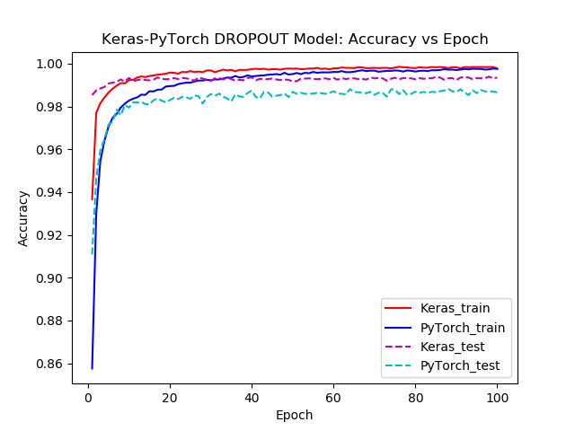
Figure1: Keras and PyTorch implemented models Accuracy vs Epochs curves
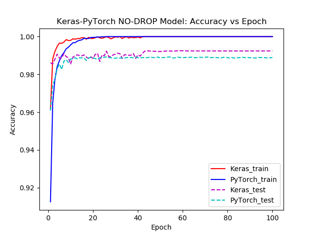
Figure2: Keras and PyTorch with NO Dropout layers: Accuracy vs Epochs curves
The results are summarized in Table 1. Testing was done by averaging the results over 10 iterrations of 100 epochs. Notice the difference of the Standard Deviations between Drop and No-Drop approaches. It turns out that we can depend on a network with Dropout Layers to be consistently better that one that does not!
| Approach | Standard Deviations | |||
|---|---|---|---|---|
| Train Acc | Train Loss | Test Acc | Test Loss | |
| PyTorch-Drop | 99.37 +- 0.0163 | 0.04838 | 98.47 +- 0.00101 | 0.00000001 |
| PyTorch-NO-Drop | 99.99 +- 0.009796 | 0.01794 | 98.23 +- 0.00342 | 0.00000994 |
| Keras-Drop | 99.64 +- 0.0068 | 0.02249 | 99.32 +- 0.00120 | 0.00680591 |
| Keras-NO-Drop | 99.99 +- 0.004062 | 0.01346 | 99.22 +- 0.00171 | 0.01140602 |
Table 1: Standard Deviations for the apporaches
So… an 0.1 and 0.24 Accuracy Improvement. Per-cent…
It seems the results are not especially staggering. But we need to consider a number of factor playing into this.
- The dataset
- The relative simplicity of the network
- The size of the test set
DataSet: The Data is the key factor of any NN’s design. We specifically design our networks to capture the intricacies of the data that describe our problem. For example object recognition can require a different approach than segmentation, financial forecast is also different than training a network to play a game. It seems that not all data or problems are equal. More elaborate data or difficult tasks require deeper and more intricate networks (i.e recurrent). MNIST character recognition is quite simple in this regard. We are provided with a well crafted data set, where each character is a black drawing of a number over a white 28x28 frame. So its easy to spot and identify and rather homogeneous.
Task Simplicity: Also, the task is straightforward: identify which character is being shown! So, a simple network should do the trick, and it does. Th network used, for which you can find the code in link at the end of this page, is a simple, sequential network, with the following layer structure:
- 2D Convolutional
- 2D Convolutional
- Max Pooling
- Dropout
- Linear
- Dropout
- SoftMax output
While this could seem not-so-simple, it is as far as NN’s go.
Test Set: Finally, we need to consider the size and structure of the test set. Again, our test set is not drastically different than our training set; if it were, as a lot of other real-life data set are, not using Drop out Layers would have a larger impact. The size of the test set also plays a role, in that a 0.1% over 10000 might not seem a lot, it is 10 characters erroneously identified. That is 3 4 digit pin attempts rejected; turns out to be important when aliens are after you, and you are trying to get the blast door open. That inconvenience could have been avoided with the simple use Of Dropout Layers!
A note on the Frameworks
Installation: Both Keras and PyTorch are quite easy to install and use, with Keras being slightly more demanding for user of older Linux Distributions such as 14.04. And by more demanding I mean one has to install an older version of Tensorflow, because the latest and greatest also requires later versions of Ubuntu. Which in terms means you have to search and specify the distribution you want and then install Keras; terrifying, I know. PyTorch on the other hand plays out of the box, just follow the instructions on the official site.
Usability: Here the medal goes to Keras, with its lego-like approach. To make a model you just have to declare the overall architecture i.e sequential and then feed the layers one as input to another; just like lego blocks! Add to that the very nice data loaders they have implemented into very handy libraries and it quickly becomes a data science aficionado’s best friend. This is ofcourse not to say that PyTorch is cumbersome to use. On the contrary. But it still requires a bit more adapting to. Here you first have to declare the layers you want to use in your model, then arrange them hierarchically inside a function, usually called “forward( **args)”, which you will then call for forward passing to your network. You also have to declare an gradient descent optimizer, to speed training convergence. After that, you have to “manually” define the training procedure; much less scary than it sounds, though. You just have to call the forward function previously defined, then call a predefined function to compute the loss of the forward pass. Based on this loss you then call a loss.backward() function, which fortunately is already implemented, to automatically compute the backpropagation gradients we need to properly fit our network. Finally, you tell your network to take a step towards “convergence” and repeat this whole procedure for all your train data set!
While these may seem a lot of steps and quite verbose, it is easy to learn and gives you quite a bit more freedom to try interesting techniques. Now, compare that with Keras’ model.fit(**args). That is all that is needed to train a compiled model in Keras. That’s it; just provide the arguments like favorite optimizer, batch size etc and you are good to go!
Performance: Now here things are interesting. It again seems like Keras comes ahead, as it take less epochs to reach peek accuracy and displays overall better Accuracy on testing, a whooping 0.9%. Granted a 0.9% percent does not sound much but it can make a difference especially on very large data sets and on, well, costly decisions. This might be because Keras uses a more mature backend, Tensorflow, that features better numerical stability or better implementation of gradient computation etc or some slight mismatch in mimicking that architecture in PyTorch on my behalf.
Future Comparison Post
This was a somewhat rushed comparison between the use of these 2 frameworks, as I aim to do a more length and detailed post on their quirks and perks!
Code
You can find the code for the network, in both frameworks here!
MNIST Recognition Nets used, in Keras/PyTorch